【特征提取】胎儿心电信号提取含Matlab源码

1 简介

本系统介绍了在MATLAB平台上,利用其提供的M语言和其他工具从母体腹腔信号中提取胎儿心电信号。

2 部分代码

%% Init
% clear all; close all;
Fs = 4e3;
Time = 40;
NumSamp = Time * Fs;
load Hd;
%% Mom's Heartbeat
% In this example, we shall simulate the shapes of the electrocardiogram
% for both the mother and fetus. The following commands create an
% electrocardiogram signal that a mother's heart might produce assuming
% a 4000 Hz sampling rate. The heart rate for this signal is approximately
% 89 beats per minute, and the peak voltage of the signal is 3.5 millivolts.
x1 = 3.5*ecg(2700).'; % gen synth ECG signal
y1 = sgolayfilt(kron(ones(1,ceil(NumSamp/2700)+1),x1),0,21); % repeat for NumSamp length and smooth
n = 1:Time*Fs';
del = round(2700*rand(1)); % pick a random offset
mhb = y1(n + del)'; %construct the ecg signal from some offset
t = 1/Fs:1/Fs:Time';
subplot(3,3,1); plot(t,mhb);
axis([0 2 -4 4]);
grid;
xlabel('Time [sec]');
ylabel('Voltage [mV]');
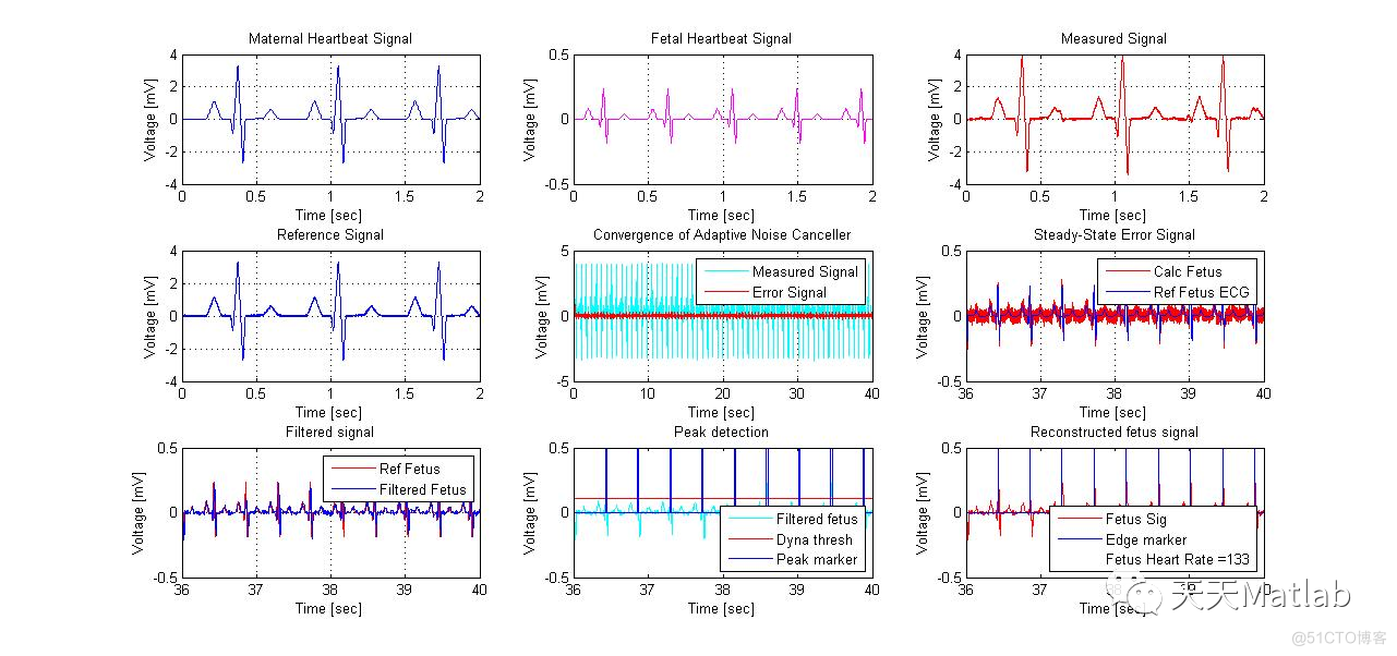
title('Maternal Heartbeat Signal');
%% Fetus Heartbeat
% The heart of a fetus beats noticeably faster than that of its mother,
% with rates ranging from 120 to 160 beats per minute. The amplitude of the
% fetal electrocardiogram is also much weaker than that of the maternal
% electrocardiogram. The following series of commands creates an electrocardiogram
% signal corresponding to a heart rate of 139 beats per minute and a peak voltage
% of 0.25 millivolts.
x2 = 0.25*ecg(1725);
y2 = sgolayfilt(kron(ones(1,ceil(NumSamp/1725)+1),x2),0,17);
del = round(1725*rand(1));
fhb = y2(n + del)';
subplot(3,3,2); plot(t,fhb,'m');
axis([0 2 -0.5 0.5]);
grid;
xlabel('Time [sec]');
ylabel('Voltage [mV]');
title('Fetal Heartbeat Signal');
%% The measured signal
% The measured fetal electrocardiogram signal from the abdomen of the mother is
% usually dominated by the maternal heartbeat signal that propagates from the
% chest cavity to the abdomen. We shall describe this propagation path as a linear
% FIR filter with 10 randomized coefficients. In addition, we shall add a small
% amount of uncorrelated Gaussian noise to simulate any broadband noise sources
% within the measurement. Can you determine the fetal heartbeat rate by looking
% at this measured signal?
Wopt = [0 1.0 -0.5 -0.8 1.0 -0.1 0.2 -0.3 0.6 0.1];
%Wopt = rand(1,10);
d = filter(Wopt,1,mhb) + fhb + 0.02*randn(size(mhb));
subplot(3,3,3); plot(t,d,'r');
axis([0 2 -4 4]);
%axis tight;
grid;
xlabel('Time [sec]');
ylabel('Voltage [mV]');
title('Measured Signal');
%% Measured Mom's heartbeat
% The maternal electrocardiogram signal is obtained from the chest of the mother.
% The goal of the adaptive noise canceller in this task is to adaptively remove the
% maternal heartbeat signal from the fetal electrocardiogram signal. The canceller
% needs a reference signal generated from a maternal electrocardiogram to perform this
% task. Just like the fetal electrocardiogram signal, the maternal electrocardiogram
% signal will contain some additive broadband noise.
x = mhb + 0.02*randn(size(mhb));
subplot(3,3,4); plot(t,x);
axis([0 2 -4 4]);
grid;
xlabel('Time [sec]');
ylabel('Voltage [mV]');
title('Reference Signal');
%% Applying the adaptive filter
% The adaptive noise canceller can use almost any adaptive procedure to perform its task.
% For simplicity, we shall use the least-mean-square (LMS) adaptive filter with 15
% coefficients and a step size of 0.00007. With these settings, the adaptive noise canceller
% converges reasonably well after a few seconds of adaptation--certainly a reasonable
% period to wait given this particular diagnostic application.
h = adaptfilt.lms(15, 0.001);
[y,e] = filter(h,x,d);
% [y,e] = FECG_detector(x,d);
subplot(3,3,5); plot(t,d,'c',t,e,'r');
%axis([0 7.0 -4 4]);
grid;
xlabel('Time [sec]');
ylabel('Voltage [mV]');
title('Convergence of Adaptive Noise Canceller');
legend('Measured Signal','Error Signal');
%% Recovering the fetus' hearbeat
% The output signal y(n) of the adaptive filter contains the estimated maternal
% heartbeat signal, which is not the ultimate signal of interest. What remains in the
% error signal e(n) after the system has converged is an estimate of the fetal heartbeat
% signal along with residual measurement noise.
subplot(3,3,6); plot(t,e,'r'); hold on; plot(t,fhb,'b');
axis([Time-4 Time -0.5 0.5]);
grid on;
xlabel('Time [sec]');
ylabel('Voltage [mV]');
title('Steady-State Error Signal');
legend('Calc Fetus','Ref Fetus ECG');
%% Counting the peaks to detect the heart rate
% The idea is to clean up the signal, andthen set some dynamic threshold, so that any signal
% crossing the threshold is considered a peak. The peaks can be counted per time window.
%[num,den] = fir1(100,100/2000);
filt_e = filter(Hd,e);
subplot(3,3,7); plot(t,fhb,'r'); hold on; plot(t,filt_e,'b');
axis([Time-4 Time -0.5 0.5]);
grid on;
xlabel('Time [sec]');
ylabel('Voltage [mV]');
title('Filtered signal');
legend('Ref Fetus','Filtered Fetus');
thresh = 4*mean(abs(filt_e))*ones(size(filt_e));
peak_e = (filt_e >= thresh);
edge_e = (diff([0; peak_e]) >0);
subplot(3,3,8); plot(t,filt_e,'c'); hold on; plot(t,thresh,'r'); plot(t,peak_e,'b');
xlabel('Time [sec]');
ylabel('Voltage [mV]');
title('Peak detection');
legend('Filtered fetus','Dyna thresh','Peak marker', 'Location','SouthEast');
axis([Time-4 Time -0.5 0.5]);
subplot(3,3,9); plot(t,filt_e,'r'); hold on; plot(t,edge_e,'b'); plot(0,0,'w');
fetus_calc = round((60/length(edge_e(16001:end))*Fs)* sum(edge_e(16001:end)));
fetus_bpm = ['Fetus Heart Rate =' mat2str(fetus_calc)];
xlabel('Time [sec]');
ylabel('Voltage [mV]');
title('Reconstructed fetus signal');
legend('Fetus Sig','Edge marker',fetus_bpm, 'Location','SouthEast');
axis([Time-4 Time -0.5 0.5]);

3 仿真结果

4 参考文献

[1]宋盟春, & 熊念. (2014). 基于匹配滤波的胎儿心电信号检测系统的研究与设计. 中国医疗器械信息, 20(3), 5.

博主简介：擅长智能优化算法、神经网络预测、信号处理、元胞自动机、图像处理、路径规划、无人机等多种领域的Matlab仿真，相关matlab代码问题可私信交流。

部分理论引用网络文献，若有侵权联系博主删除。