1 内容介绍
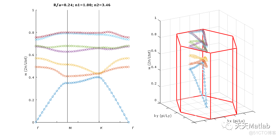
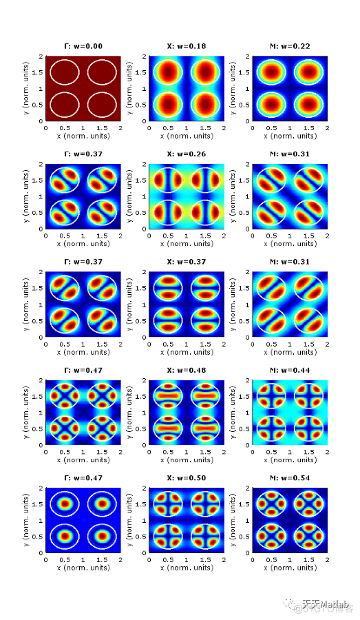
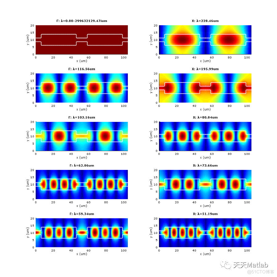
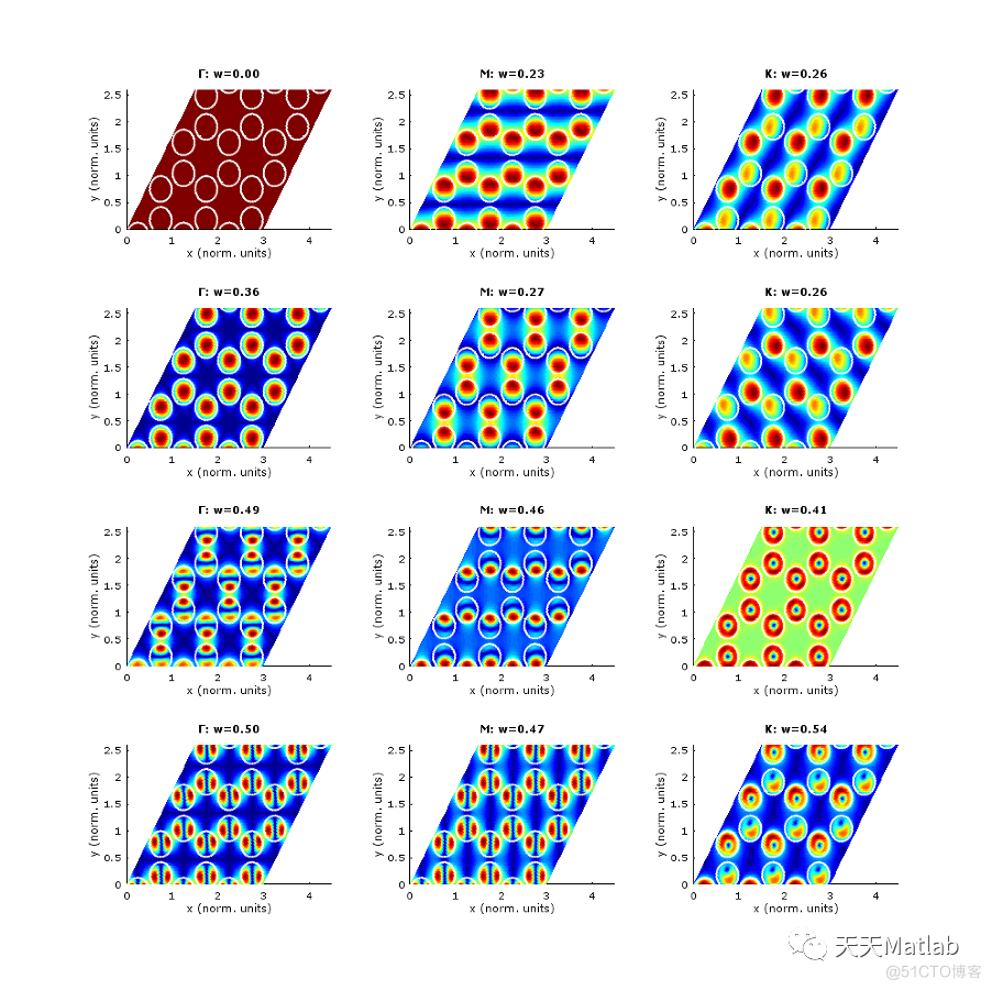
为了了解电磁波在光子晶体中的传输特性,用MATLAB与时域有限差分法把电磁波在真空与光子晶体中的传播实时可视化,并给出了场的空间静态分布.数值模拟的结果表明,禁带中的波被光子晶体控制,其能量分布在介质柱中,并观察到了电磁波局域化现象.
2 部分代码
clear alllose allclc%%%%%%%%%%%%%%%%%%%%%%%%%%%%%%%%%%%%%%%%%%%%%%%%%%%%%%%%%%%%%%%%%%%%%%%%%%%%%%%
%%%%%%%%%%%%%%%%%%%%%%%%%%%%%%%% Constants %%%%%%%%%%%%%%%%%%%%%%%%%%%%%%%%%%%%%
%%%%%%%%%%%%%%%%%%%%%%%%%%%%%%%%%%%%%%%%%%%%%%%%%%%%%%%%%%%%%%%%%%%%%%%%%%%%%%%%
c=2.99792458e8;
%%%%%%%%%%%%%%%%%%%%%%%%%%%%%%%%%%%%%%%%%%%%%%%%%%%%%%%%%%%%%%%%%%%%%%%%%%%%%%%%
%%%%%%%%%%%%%%%%%%%%%%%%%% Plotting parameter %%%%%%%%%%%%%%%%%%%%%%%%%%%%%%%%%
%%%%%%%%%%%%%%%%%%%%%%%%%%%%%%%%%%%%%%%%%%%%%%%%%%%%%%%%%%%%%%%%%%%%%%%%%%%%%%%%
band=1;
Field=1;
Epsilon=0;
AAbs=1; %% Plot abs(E)
RReal=0; %% Plot real(E)
IImag=0; %% Plot imag(E)
%%%%%%%%%%%%%%%%%%%%%%%%%%%%%%%%%%%%%%%%%%%%%%%%%%%%%%%%%%%%%%%%%%%%%%%%%%%%%%%%
%%%%%%%%%%%%%%%%%%%%%%%%%%%%%%%% Parameters %%%%%%%%%%%%%%%%%%%%%%%%%%%%%%%%%%%%
%%%%%%%%%%%%%%%%%%%%%%%%%%%%%%%%%%%%%%%%%%%%%%%%%%%%%%%%%%%%%%%%%%%%%%%%%%%%%%%%
hex=1;
comb=0;
TM=0;
TE=1;
Nx=32; % number of points on the x grid % has to be a power of 2 (32,64,128,256,512,...)
Ny=32; % number of points on the y grid % has to be a power of 2 (32,64,128,256,512,...)
NGx=10; % number of harmonics % has to be 2 times -1 smaller than x
NGy=11; % number of harmonics % has to be 2 times -1 smaller than y
Nkx=10; % number of points on the k space for the dispersion
Nky=Nkx; % number of points on the k space for the dispersion
nmodes=5; % number of solutions asked
Np=3; % number of period to plot for the Field
n1 =1; %% optical index material 1
n2 = sqrt(12); %% optical index material 2
NormUnits=1;
%%%%%%%%%%%%%%%%%%%%%%%%%%%%%%%%%%%%%%%%%%%%%%%%%%%%%%%%%%%%%%%%%%%%%%%%%%%%%%%%
%%%%%%%%%%%%%%%%%%%%%%% Building of the index Geometry %%%%%%%%%%%%%%%%%%%%%%%%%
%%%%%%%%%%%%%%%%%%%%%%%%%%%%%%%%%%%%%%%%%%%%%%%%%%%%%%%%%%%%%%%%%%%%%%%%%%%%%%%%
if NormUnits==1
L=1;
elseif NormUnits==0
L=1e-6;
end
Lx=L;
Ly=L*sqrt(3)/2;
a1=Lx*[1 0];
a2=Lx*[ 1/2 sqrt(3)/2 ];
count=1;
for jj=0:Nx-1,
for j=0:Ny-1,
AAA(count,:) = jj*a1/(Nx-1) + j*a2/(Ny-1) ;
count=count+1;
end
end
Xhex=reshape(AAA(:,1),Ny,Nx);
Yhex=reshape(AAA(:,2),Ny,Nx);
dx=Xhex(1,2)-Xhex(1,1);
dy=Yhex(2,1)-Yhex(1,1);
if (hex==1) && (comb==1) || (hex==0) && (comb==0)
display('Error: Select hexagonal lattice or honey-comb lattice')
break
end
if hex==1
a=0.3;%0.495;
idx1 = ( (Xhex-Lx*3/4).^2 + (Yhex-Ly/2).^2 ) < (a*L)^2;
idx2 = ( (Xhex-Lx*3/4+Lx/2).^2 + (Yhex-Ly/2+Ly).^2 ) < (a*L)^2;
idx3 = ( (Xhex-Lx*3/4-Lx/2).^2 + (Yhex-Ly/2-Ly).^2 ) < (a*L)^2;
idx4 = ( (Xhex-Lx*3/4-Lx).^2 + (Yhex-Ly/2).^2 ) < (a*L)^2;
idx5 = ( (Xhex-Lx*3/4+Lx).^2 + (Yhex-Ly/2).^2 ) < (a*L)^2;
idx=idx1+idx2+idx3+idx4+idx5;
eps = idx*n2^2 + (1-idx)*n1^2 ;
end
if comb==1
a=0.24;
idx1a = ( (Xhex-Lx*3/4).^2 + (Yhex-Ly/5).^2 ) < (a*L)^2;
idx1b = ( (Xhex-Lx*3/4+Lx/2).^2 + (Yhex-Ly/5-Lx/sqrt(3)+Ly).^2 ) < (a*L)^2;
idx2a = ( (Xhex-Lx*3/4).^2 + (Yhex-Ly/5-Lx/sqrt(3)).^2 ) < (a*L)^2;
idx2b = ( (Xhex-Lx*3/4-Lx/2).^2 + (Yhex-Ly/5-Ly).^2 ) < (a*L)^2;
idx=idx1a+idx1b+idx2a+idx2b;
eps = idx*n2^2 + (1-idx)*n1^2 ;
end
%%%%%%%%%%%%%%%%%%%%%%%%%%%%%%%%%%%%%%%%%%%%%%%%%%%%%%%%%%%%%%%%%%%%%%%%%%%%%%%%
%%%%%%%%%%%%%%%%%%%%%%%%% Reciprocal lattice vectors %%%%%%%%%%%%%%%%%%%%%%%%%%%
%%%%%%%%%%%%%%%%%%%%%%%%%%%%%%%%%%%%%%%%%%%%%%%%%%%%%%%%%%%%%%%%%%%%%%%%%%%%%%%%
NGx = 2*floor(NGx/2); %% round to lower even number
NGy = 2*floor(NGy/2); %% round to lower even number
b1=2*pi/Lx*[1 -sqrt(3)/3];
b2=2*pi/Lx*[0 2*sqrt(3)/3];
count=1;
GGG=[];
for jj=-NGx:NGx
for j=-NGy:NGy
GGG(count,:)=jj*b1+j*b2;
count=count+1;
end
end
Gxhex=reshape(GGG(:,1),2*NGy+1,2*NGx+1);
Gyhex=reshape(GGG(:,2),2*NGy+1,2*NGx+1);
%%%%%%%%%%%%%%%%%%%%%%%%%%%%%%%%%%%%%%%%%%%%%%%%%%%%%%%%%%%%%%%%%%%%%%%%%%%%%%%%
%%%%%%%%%%%%%%%%%%%%%%%%%% Hexagonal Fourier Transform %%%%%%%%%%%%%%%%%%%%%%%%%
%%%%%%%%%%%%%%%%%%%%%%%%%%%%%%%%%%%%%%%%%%%%%%%%%%%%%%%%%%%%%%%%%%%%%%%%%%%%%%%%
Gamma=1./eps;
f=Gamma;
for jj=1:length(Gxhex(1,:))
for j=1:length(Gyhex(:,1))
whex = exp( -1i*( Gxhex(1,jj) *(Xhex-Xhex(1))*(Nx-1)/Nx + ( Gyhex(j,jj) )*(Yhex-Yhex(1))*(Ny-1)/Ny ) );
Ghex(j,jj) = sum(sum(f.*whex));
end
end
Gammak = Ghex*dx*dy/Lx/Ly ;
%%%%%%%%%%%%%%%%%%%%%%%%%%%%%%%%%%%%%%%%%%%%%%%%%%%%%%%%%%%%%%%%%%%%%%%%%%%%%%%%
%%%%%%%%%%%%%%%% Building of the reciproque lattice vector %%%% again %%%%%%%%%%
%%%%%%%%%%%%%%%%%%%%%%%%%%%%%%%%%%%%%%%%%%%%%%%%%%%%%%%%%%%%%%%%%%%%%%%%%%%%%%%%
count=1;
GGG=[];
for jj=-NGx/2:NGx/2,
for j=-NGy/2:NGy/2,
GGG(count,:)=jj*b1+j*b2;
count=count+1;
end
end
Gxhex=reshape(GGG(:,1),NGy+1,NGx+1);
Gyhex=reshape(GGG(:,2),NGy+1,NGx+1);
NGx=length(Gxhex(1,:));
NGy=length(Gyhex(:,1));
NG=NGx*NGy;
%%%%%%%%%%%%%%%%%%%%%%%%%%%%%%%%%%%%%%%%%%%%%%%%%%%%%%%%%%%%%%%%%%%%%%%%%%%%%%%%
%%%%%%%%%%%%%%%%%%%%%%%%%% Building of k-space vector %%%%%%%%%%%%%%%%%%%%%%%%%%
%%%%%%%%%%%%%%%%%%%%%%%%%%%%%%%%%%%%%%%%%%%%%%%%%%%%%%%%%%%%%%%%%%%%%%%%%%%%%%%%
kx=linspace( 0 , pi/L , Nkx)*2/3;
ky=linspace( 0 , pi/Ly , Nky);
k=[
ky'*0 ky'
kx' ky(end)+kx'*0
sort(kx,'descend')' sort(ky,'descend')'
];
%%%%%%%%%%%%%%%%%%%%%%%%%%%%%%%%%%%%%%%%%%%%%%%%%%%%%%%%%%%%%%%%%%%%%%%%%%%%%%%%
%%%%%%%%%%%%%%%%%%%%%%%%%%%%%%%%%%%%%%%%%%%%%%%%%%%%%%%%%%%%%%%%%%%%%%%%%%%%%%%%
%%%%%%%%%%%%%%%%%%%%%%%%%%%%%%%%%%%%%%%%%%%%%%%%%%%%%%%%%%%%%%%%%%%%%%%%%%%%%%%%
%%%%%%%%%%%%%%%%%%%%%%% NOTHING TO CHANGE ANYMORE!!! %%%%%%%%%%%%%%%%%%%%%%%%%%%
%%%%%%%%%%%%%%%%%%%%%%%%%%%%%%%%%%%%%%%%%%%%%%%%%%%%%%%%%%%%%%%%%%%%%%%%%%%%%%%%
%%%%%%%%%%%%%%%%%%%%%%%%%%%%%%%%%%%%%%%%%%%%%%%%%%%%%%%%%%%%%%%%%%%%%%%%%%%%%%%%
%%%%%%%%%%%%%%%%%%%%%%%%%%%%%%%%%%%%%%%%%%%%%%%%%%%%%%%%%%%%%%%%%%%%%%%%%%%%%%%%
%%%%%%%%%%%%%%%%%%%%%%%%%%%%%%%%%%%%%%%%%%%%%%%%%%%%%%%%%%%%%%%%%%%%%%%%%%%%%%%%
if (TE==1 && TM==1) || (TE==0 && TM==0)
display('Error: Select "TM" or "TE"')
break
end
%%%%%%%%%%%%%%%%%%%%%%%%%%%%%%%%%%%%%%%%%%%%%%%%%%%%%%%%%%%%%%%%%%%%%%%%%%%%%%%%
%%%%%%%% Building first part of Hamitonian that is not depending on k %%%%%%%%%%
%%%%%%%%%%%%%%%%%%%%%%%%%%%%%%%%%%%%%%%%%%%%%%%%%%%%%%%%%%%%%%%%%%%%%%%%%%%%%%%%
HHH=zeros(NGy,NGx,NGy,NGx);
for ix=1:NGx
for jx=1:NGx
for iy=1:NGy
for jy=1:NGy
HHH(iy,ix,jy,jx) = Gammak(iy-jy+NGy,ix-jx+NGx );
end
end
end
end
%%%%%%%%%%%%%%%%%%%%%%%%%%%%%%%%%%%%%%%%%%%%%%%%%%%%%%%%%%%%%%%%%%%%%%%%%%%%%%%%
for i=1:length(k(:,1))
[psi,f0]=PhC2D_hex_PWE_f(Xhex,Yhex,Gxhex,Gyhex,k(i,:),HHH,nmodes,TE,TM);
E(:,:,:,i)=psi;
if NormUnits==1
FF(:,i) = f0 * Lx / (2*pi);
elseif NormUnits==0
FF(:,i) = f0 * c / (2*pi) *1e-12; % Convert in THz
lambda(:,i)=2*pi./f0*1e6; % Convert in wavelength (um)
end
end
%%%%%%%%%%%%%%%%%%%%%%%%%%%%%%%%%%%%%%%%%%%%%%%%%%%%%%%%%%%%%%%%%%%%%%%%%%%%%%%%
%%%%%%%%%%%%%%%%%%%%%%%%%%%%%%%%% Figures %%%%%%%%%%%%%%%%%%%%%%%%%%%%%%%%%%%%%%
%%%%%%%%%%%%%%%%%%%%%%%%%%%%%%%%%%%%%%%%%%%%%%%%%%%%%%%%%%%%%%%%%%%%%%%%%%%%%%%%
if AAbs==1
EE=abs(E);
end
if RReal==1
EE=real(E);
end
if IImag==1
EE=imag(E);
end
if NormUnits==0
Xhex=Xhex*1e6;
Yhex=Yhex*1e6;
Lx=Lx*1e6;
Ly=Ly*1e6;
k=k*1e-6;
end
if Field==1
if TM==1 && TE==0
figure('position',[100 50 1000 1000],'name','Ez');
elseif TE==1 && TM==0
figure('position',[100 50 1000 1000],'name','Exy');
end
colormap(jet)
for ii=0:nmodes-1
for i=1:Np
for j=1:Np
subplot(nmodes,3,1+3*ii)
hold on
pcolor( Xhex+(i-1+(j-1)/2)*Lx , Yhex+(j-1)*Ly , EE(:,:,ii+1,1) )
contour( Xhex+(i-1+(j-1)/2)*Lx , Yhex+(j-1)*Ly ,abs(eps),1,'linewidth',2,'linecolor','w')
end
end
shading flat
%colorbar
if RReal==1 || IImag==1
caxis([-1 1])
elseif AAbs==1
caxis([0 1])
end
if NormUnits==1
title(strcat('\Gamma: w=' , num2str(FF(1+ii,1), '%.2f') ))
xlabel('x (norm. units)')
ylabel('y (norm. units)')
elseif NormUnits==0
title(strcat('\Gamma: \lambda=' , num2str(lambda(1+ii,1), '%.2f') , 'um' ))
xlabel('x (um)')
ylabel('y (um)')
end
xlim([0 1.5*Np*Lx])
ylim([0 Np*Ly])
end
for ii=0:nmodes-1
for i=1:Np
for j=1:Np
subplot(nmodes,3,2+3*ii)
hold on
pcolor( Xhex+(i-1+(j-1)/2)*Lx , Yhex+(j-1)*Ly , EE(:,:,ii+1,1*Nkx) )
contour( Xhex+(i-1+(j-1)/2)*Lx , Yhex+(j-1)*Ly ,abs(eps),1,'linewidth',2,'linecolor','w')
end
end
shading flat
%colorbar
if RReal==1 || IImag==1
caxis([-1 1])
elseif AAbs==1
caxis([0 1])
end
if NormUnits==1
title(strcat('M: w=' , num2str(FF(1+ii,length(k)/3), '%.2f') ))
xlabel('x (norm. units)')
ylabel('y (norm. units)')
elseif NormUnits==0
title(strcat('M: \lambda=' , num2str(lambda(1+ii,length(k)/3), '%.2f') , 'um' ))
xlabel('x (um)')
ylabel('y (um)')
end
xlim([0 1.5*Np*Lx])
ylim([0 Np*Ly])
end
for ii=0:nmodes-1
for i=1:Np
for j=1:Np
subplot(nmodes,3,3+3*ii)
hold on
pcolor( Xhex+(i-1+(j-1)/2)*Lx , Yhex+(j-1)*Ly , EE(:,:,ii+1,2*Nkx) )
contour( Xhex+(i-1+(j-1)/2)*Lx , Yhex+(j-1)*Ly ,abs(eps),1,'linewidth',2,'linecolor','w')
end
end
shading flat
%colorbar
if RReal==1 || IImag==1
caxis([-1 1])
elseif AAbs==1
caxis([0 1])
end
if NormUnits==1
title(strcat('K: w=' , num2str(FF(1+ii,length(k)*2/3), '%.2f') ))
xlabel('x (norm. units)')
ylabel('y (norm. units)')
elseif NormUnits==0
title(strcat('K: \lambda=' , num2str(lambda(1+ii,length(k)*2/3), '%.2f') , 'um' ))
xlabel('x (um)')
ylabel('y (um)')
end
xlim([0 1.5*Np*Lx])
ylim([0 Np*Ly])
end
end
%%%%%%%%%%%%%%%%%%%%%%%%%%%%%%%%%%%%%%%%%%%%%%%%%%%%%%%%%%%%%%%%%%%%%%%%%%%%%%%%
if Epsilon==1
figure('position',[1100 50 500 400])
subplot(111)
hold on
for i=1:Np
for j=1:Np
pcolor( Xhex+(i-1+(j-1)/2)*Lx , Yhex+(j-1)*Ly , real(eps) )
end
end
shading flat
colormap(jet)
c=colorbar;
title(c,'Epsilon')
if NormUnits==1
xlabel('x (norm. units)')
ylabel('y (norm. units)')
elseif NormUnits==0
xlabel('x (um)')
ylabel('y (um)')
end
%axis equal
end
%%%%%%%%%%%%%%%%%%%%%%%%%%%%%%%%%%%%%%%%%%%%%%%%%%%%%%%%%%%%%%%%%%%%%%%%%%%%%%%%
if band==1
figure('position',[50 570 900 450])
subplot(1,2,1)
hold on;%grid on;
plot(0:length(k)-1,real(FF(1:nmodes,:))','o-')
yscale=get(gca,'ylim');
xlim([0 length(k)-1])
plot( [1/3*length(k) 1/3*length(k)] , yscale , 'k')
plot( [2/3*length(k) 2/3*length(k)] , yscale , 'k')
plot( [3/3*length(k) 3/3*length(k)] , yscale , 'k')
text(0/3*length(k) , -0.05*yscale(2) , ' \Gamma')
text(1/3*length(k) , -0.05*yscale(2) , ' M' )
text(2/3*length(k) , -0.05*yscale(2) , ' K' )
text(3/3*length(k) , -0.05*yscale(2) , ' \Gamma')
%xlabel('k')
set(gca,'xticklabel',[])
if NormUnits==1
ylabel('w (2\pi/Ltot)')
elseif NormUnits==0
ylabel('f (THz)')
end
title(strcat('R/a=',num2str(a),'; n1=',num2str(n1,'%.2f'),'; n2=',num2str(n2,'%.2f') ))
%%%%%%%%%%%%%%%%%%%%%%%%%%%%%%%%%%%%%%%%%%%%%%%%%%%%%%%%%%%%%%%%%%%%%%%%
subplot(1,2,2)
hold on;grid on;
LW=2;
for i=1:nmodes
plot3( k(:,1)*Lx/pi , k(:,2)*Ly/pi , real(FF(i,:))','o-')
end
set(gca,'xticklabel',[])
set(gca,'yticklabel',[])
xlabel('kx (pi/Lx)')
ylabel('ky (pi/Ly)')
if NormUnits==1
zlabel('w (2\pi/Ltot)')
elseif NormUnits==0
zlabel('f (THz)')
end
view(-30,15)
plot3( [-1 1]*2/3 , +[1 1] , [0 0] ,'r', 'linewidth',LW )
plot3( [-1 1]*2/3 , -[1 1] , [0 0] ,'r', 'linewidth',LW )
plot3( +[1 2]*2/3 , +[1 0] , [0 0] ,'r', 'linewidth',LW )
plot3( +[1 2]*2/3 , -[1 0] , [0 0] ,'r', 'linewidth',LW )
plot3( -[2 1]*2/3 , -[0 1] , [0 0] ,'r', 'linewidth',LW )
plot3( -[2 1]*2/3 , +[0 1] , [0 0] ,'r', 'linewidth',LW )
plot3( [-1 1]*2/3 , +[1 1] , [1 1]*max(real(FF(nmodes,:))) ,'r', 'linewidth',LW )
plot3( [-1 1]*2/3 , -[1 1] , [1 1]*max(real(FF(nmodes,:))) ,'r', 'linewidth',LW )
plot3( +[1 2]*2/3 , +[1 0] , [1 1]*max(real(FF(nmodes,:))) ,'r', 'linewidth',LW )
plot3( +[1 2]*2/3 , -[1 0] , [1 1]*max(real(FF(nmodes,:))) ,'r', 'linewidth',LW )
plot3( -[2 1]*2/3 , -[0 1] , [1 1]*max(real(FF(nmodes,:))) ,'r', 'linewidth',LW )
plot3( -[2 1]*2/3 , +[0 1] , [1 1]*max(real(FF(nmodes,:))) ,'r', 'linewidth',LW )
plot3( +[1 1]*2/3 , +[1 1] , [0 1]*max(real(FF(nmodes,:))) ,'r', 'linewidth',LW )
plot3( +[1 1]*2/3 , -[1 1] , [0 1]*max(real(FF(nmodes,:))) ,'r', 'linewidth',LW )
plot3( -[1 1]*2/3 , +[1 1] , [0 1]*max(real(FF(nmodes,:))) ,'r', 'linewidth',LW )
plot3( -[1 1]*2/3 , -[1 1] , [0 1]*max(real(FF(nmodes,:))) ,'r', 'linewidth',LW )
plot3( +2*[1 1]*2/3 ,0*[1 1] , [0 1]*max(real(FF(nmodes,:))) ,'r', 'linewidth',LW )
plot3( -2*[1 1]*2/3 ,0*[1 1] , [0 1]*max(real(FF(nmodes,:))) ,'r', 'linewidth',LW )
end
%%%%%%%%%%%%%%%%%%%%%%%%%%%%%%%%%%%%%%%%%%%%%%%%%%%%%%%%%%%%%%%%%%%%%%%%%%%%%%%%
%%%%%%%%%%%%%%%%%%%%%%%%%%%%%%%%%%% END %%%%%%%%%%%%%%%%%%%%%%%%%%%%%%%%%%%%%%%%
%%%%%%%%%%%%%%%%%%%%%%%%%%%%%%%%%%%%%%%%%%%%%%%%%%%%%%%%%%%%%%%%%%%%%%%%%%%%%%%%
3 运行结果


4 参考文献
[1]王磊. 任意形状二维介质光子晶体特性研究[D]. 电子科技大学, 2008.
[2]荣垂才, 闫珂柱, 谢应茂. 二维光子晶体中场的分布[J]. 激光技术, 2008.
