主要介绍箱线图(Box-plot)和利用Matlab绘制箱线图。
1、箱线图介绍
统计指标一般包括:四分位数、均值、中位数、众数、方差、标准差等,箱线图作为一种数据统计的方法,内容包括:最小值,第一分位,中位数,第三分位数,最大值。


编辑
箱线图于1977年由美国著名统计学家约翰·图基(John Tukey)发明,能够明确的展示离群点的信息,同时能够让我们了解数据是否对称,数据如何分组、数据的峰度。
箱线图(Box-plot)是一种用于显示一组数据分散情况的统计图,多用于多组数据的比较,相对于直方图,既可以节省空间,还可以展示更多信息(如均值、四分位数等)。
箱线图包含数学统计量,能够分析不同类别数据各层次水平差异,还可以揭示数据间离散程度、异常值、分布差异等。
箱线图内容详细介绍:


编辑
【注】图片来自你似乎来到了没有知识存在的荒原 - 知乎
四分位数:
一组数据按照从小到大顺序排列后,把该组数据四等分的数,称为四分位数。第一四分位数 (Q1)、第二四分位数 (Q2,也叫“中位数”)和第三四分位数 (Q3)分别等于该样本中所有数值由小到大排列后第25%、第50%和第75%的数字。第三四分位数与第一四分位数的差距又称四分位距(interquartile range, IQR)。
(1)第一个四分位数Q1:也称作25th百分位数,表示最小数(不是“最小值”)和数据集的中位数之间的中间数。
(2)第二四分位数Q2:也称作中位数Median/50th百分位数,表示数据集的中间值。
(3)第三四分位数Q3:也称作75th百分位数,表示数据集的中位数和最大值之间的中间值(不是“最大值”)。
(4)四分位间距IQR:第25至第75个百分点的距离。
(5)离群值:Outliers
(6)最大值max、最小值min
利用正态分布的箱线图,可以帮助理解箱线图:


编辑
【注】图片来自你似乎来到了没有知识存在的荒原 - 知乎
2 完整代码
function boxPlot3D(xx,g1,g2,quantDistribution)
%function boxPlot3D(xx,g1,g2,quantDistribution)
%--------------------------------------------------------------------------
% boxPlot3D(x) creates a three dimensional box plot of the data in x. If x
% is 3D a matrix, boxPlot3D creates one box for each column. Example,
% create a 3D matrix with normal distributions with different means:
%
% xx=randn(50,2,4)+repmat((permute([0 1 2 -2;1 2 3 4],[3 1 2])),[50,1,1]);
% boxPlot3D(xx)
%
% boxPlot3D(x,g1,g2) groups the data of x, with the grouping variables of
% g1, and g2. Example, create a 1D Matrix with different values and the
% corresponding grouping parameters:
%
% xx=randn(500,1)+linspace(0,5,500)';
% g1= [0.1*ones(250,1);0.2*ones(250,1)];
% g2= [3*ones(150,1);4*ones(150,1);5*ones(200,1)];
% boxPlot3D(xx,g1,g2)
%
% boxPlot3D(x,[],[],quantDistribution) allows the selection of the
% quantiles to select, e.g. [0 0.25 0.5 0.75 1]
% [0 0.25 0.5 0.75 1] (default) creates a box between 0.25 and 0.75
% with a line in 0.5 and two planes at 0 and 1
% connected with a dashed line. These values can be
% changed.
% [ 0 1] creates a box within the extremes of the values
% selected. These values can be changed, e.g.
% [0.25 0.75]
% [ 0.25 0.5 0.75] creates a box and a line, same as the option with
% 5 values, but will not draw the planes with the
% dashed line.
% The colours of the boxes can be changed in the code.
%--------------------------------------------------------------------------
%
%
if nargin <1
else
figure
hold on;
if ~exist('quantDistribution','var')
% Calculate the positions of the edges of the boxplot, and the
% quantiles at 25,50 75%
quantDistribution = [0 0.25 0.50 0.75 1 ];
end
if ~exist('g1','var')
% Only one parameter received, the data is in a 3D Matrix with one
% column per group.
[rows,columns,levels] = size( xx);
for counterCols = 1:columns
for counterLevs = 1:levels
% Select columns, extract positions, and call display
% The column is directly extracted from the matrix
currentColumn = xx(:,counterCols,counterLevs);
% The positions correspond to the extreme, median and 25%/75%
% positions of the distribution, these are obtained with
% quantile
currentPositions = quantile(currentColumn,quantDistribution);
display3Dbox(counterCols,counterLevs,currentPositions);
end
end
else
% Three arguments, the data and two grouping parameters
% all should be the same size. First, detect the unique cases of
% each of the grouping parameters
cases_g1=unique(g1);
cases_g2=unique(g2);
% Count how many cases there are for each dimension
num_g1 = numel(cases_g1);
num_g2 = numel(cases_g2);
% The separation may vary and not necessarily be 0,1,2,3...
width_g1 = min(diff(cases_g1));
width_g2 = min(diff(cases_g2));
for counterCols = 1:num_g1
current_g1 = cases_g1(counterCols);
address_g1 = (g1==current_g1);
for counterLevs = 1:num_g2
current_g2 = cases_g2(counterLevs);
address_g2 = (g2==current_g2);
% Select columns, extract positions, and call display
% The column is directly extracted from the matrix
currentColumn = xx((address_g1)&(address_g2));
% The positions correspond to the extreme, median and 25%/75%
% positions of the distribution, these are obtained with
% quantile
currentPositions = quantile(currentColumn,quantDistribution);
% Call the display with the extra parameters for width
display3Dbox(current_g1,current_g2,currentPositions,width_g1,width_g2);
end
end
end
view(3)
rotate3d on
axis tight
grid on
end
end
function display3Dbox(counterCols,counterLevs,currentPositions,width_g1,width_g2)
if ~exist('width_g1','var')
width_g1 = 1;
end
if ~exist('width_g2','var')
width_g2 = 1;
end
if ~exist('colourFace','var')
colourFace='red';
end
if ~exist('colourFace2','var')
colourFace2='cyan';
end
lenZStats=length(currentPositions);
% to avoid overlap between boxes, use only 35% to each dimension
x=width_g1 * 0.35*[-1 1 1 -1 -1 1 1 -1]';
y=width_g2 * 0.35*[-1 -1 1 1 -1 -1 1 1]';
% This are the parameters to create the boxes and faces
z=[1 1 1 1]';
face_Mat=[1 2 6 5;2 3 7 6;3 4 8 7;4 1 5 8;4 1 5 8;1 2 3 4; 5 6 7 8];
switch lenZStats
case 2
%----- a single box with extremes (.25 .75 / 0 1) to be plotted
vert_Mat=[counterCols+x counterLevs+y [currentPositions(1)*z;currentPositions(2)*z]];
patch('Vertices',vert_Mat,'Faces',face_Mat,'facecolor',colourFace,'edgecolor','black','linewidth',1);
case 3
%----- a central box with median (0.25 0.5 0.75)
delta=0.05*(currentPositions(3)-currentPositions(1));
vert_Mat=[counterCols+x counterLevs+y [currentPositions(1)*z;currentPositions(2)*z-delta/2]];
patch('Vertices',vert_Mat,'Faces',face_Mat,'facecolor',colourFace,'edgecolor','black','linewidth',1);
vert_Mat=[counterCols+x counterLevs+y [currentPositions(2)*z-delta/2;currentPositions(2)*z+delta/2]];
patch('Vertices',vert_Mat,'Faces',face_Mat,'facecolor',colourFace2,'edgecolor','black','linewidth',1);
vert_Mat=[counterCols+x counterLevs+y [currentPositions(2)*z+delta/2;currentPositions(3)*z-delta/2]];
patch('Vertices',vert_Mat,'Faces',face_Mat,'facecolor',colourFace,'edgecolor','black','linewidth',1);
case 5
%----- central box with extemes (0 0.25 0.5 0.75 1)
delta=0.05*(currentPositions(3)-currentPositions(1));
colourFace3=0.5*[1 1 1];
vert_Mat=[counterCols+x counterLevs+y [currentPositions(2)*z;currentPositions(3)*z-delta/2]];
patch('Vertices',vert_Mat,'Faces',face_Mat,'facecolor',colourFace,'edgecolor','black','linewidth',1);
vert_Mat=[counterCols+x counterLevs+y [currentPositions(3)*z-delta/2;currentPositions(3)*z+delta/2]];
patch('Vertices',vert_Mat,'Faces',face_Mat,'facecolor',colourFace2,'edgecolor','black','linewidth',1);
vert_Mat=[counterCols+x counterLevs+y [currentPositions(3)*z+delta/2;currentPositions(4)*z-delta/2]];
patch('Vertices',vert_Mat,'Faces',face_Mat,'facecolor',colourFace,'edgecolor','black','linewidth',1);
vert_Mat=[counterCols+x*(0.5) counterLevs+y*(0.5) [currentPositions(1)*z;currentPositions(1)*z]];
patch('Vertices',vert_Mat,'Faces',face_Mat,'facecolor',colourFace3,'edgecolor','black','linewidth',0.5);
vert_Mat=[counterCols+x*(0.5) counterLevs+y*(0.5) [currentPositions(5)*z;currentPositions(5)*z]];
patch('Vertices',vert_Mat,'Faces',face_Mat,'facecolor',colourFace3,'edgecolor','black','linewidth',0.5);
line([counterCols counterCols],[counterLevs counterLevs],[currentPositions(1) currentPositions(2)],'linewidth',0.5,'color','k','marker','.','linestyle','--')
line([counterCols counterCols],[counterLevs counterLevs],[currentPositions(4) currentPositions(5)],'linewidth',0.5,'color','k','marker','.','linestyle','--')
end
end
%delta=0.04;
%alpha(0.5);
%grid on;axis tight;rotate3d on;view(3)
3 运行结果

编辑


编辑
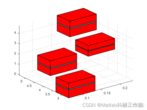

编辑
4 参考文献
部分理论引用网络文献,若有侵权联系博主删除。