Python数值方法及数据可视化

• 随机数和蒙特卡洛模拟
• 求解单一变量非线性方程
• 求解线性系统方程
• 函数的数学积分
• 常微分方程的数值解

等势线绘图和曲线：

等势线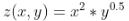 

import numpy as np
import matplotlib.pyplot as plt
from mpl_toolkits.mplot3d import Axes3D
 
x_vals = np.linspace(-5,5,20)
y_vals = np.linspace(0,10,20)
 
X,Y = np.meshgrid(x_vals,y_vals)
Z = X**2 * Y**0.5
line_count = 15
 
ax = Axes3D(plt.figure())
ax.plot_surface(X,Y,Z,rstride=1,cstride=1)
plt.show()

非线性方程的数学解：

• 一般实函数  Scipy.optimize
• fsolve函数求零点（限定只给实数解）

import scipy.optimize as so
from scipy.optimize import fsolve
 
f = lambda x:x**2-1
fsolve(f,0.5)
fsolve(f,-0.5)
fsolve(f,[-0.5,0.5])
 
 
>>>fsolve(f,-0.5,full_output=True)
>>>(array([-1.]), {'nfev': 9, 'fjac': array([[-1.]]), 'r': array([1.99999875]), 'qtf': array([3.82396337e-10]), 'fvec': array([4.4408921e-16])}, 1, 'The solution converged.')
 
>>>help(fsolve)
>>>Help on function fsolve in module scipy.optimize._minpack_py:
 
fsolve(func, x0, args=(), fprime=None, full_output=0, col_deriv=0, xtol=1.49012e-08, maxfev=0, band=None, epsfcn=None, factor=100, diag=None)
    Find the roots of a function.

    Return the roots of the (non-linear) equations defined by
    ``func(x) = 0`` given a starting estimate.

    Parameters
    ----------
    func : callable ``f(x, *args)``
        A function that takes at least one (possibly vector) argument,
        and returns a value of the same length.
    x0 : ndarray
        The starting estimate for the roots of ``func(x) = 0``.
    args : tuple, optional
        Any extra arguments to `func`.
    fprime : callable ``f(x, *args)``, optional
        A function to compute the Jacobian of `func` with derivatives
        across the rows. By default, the Jacobian will be estimated.
    full_output : bool, optional
        If True, return optional outputs.
    col_deriv : bool, optional
        Specify whether the Jacobian function computes derivatives down
        the columns (faster, because there is no transpose operation).
    xtol : float, optional
        The calculation will terminate if the relative error between two
        consecutive iterates is at most `xtol`.
    maxfev : int, optional
        The maximum number of calls to the function. If zero, then
        ``100*(N+1)`` is the maximum where N is the number of elements
        in `x0`.
    band : tuple, optional
        If set to a two-sequence containing the number of sub- and
        super-diagonals within the band of the Jacobi matrix, the
        Jacobi matrix is considered banded (only for ``fprime=None``).
    epsfcn : float, optional
        A suitable step length for the forward-difference
        approximation of the Jacobian (for ``fprime=None``). If
        `epsfcn` is less than the machine precision, it is assumed
        that the relative errors in the functions are of the order of
        the machine precision.
    factor : float, optional
        A parameter determining the initial step bound
        (``factor * || diag * x||``). Should be in the interval
        ``(0.1, 100)``.
    diag : sequence, optional
        N positive entries that serve as a scale factors for the
        variables.

    Returns
    -------
    x : ndarray
        The solution (or the result of the last iteration for
        an unsuccessful call).
    infodict : dict
        A dictionary of optional outputs with the keys:

        ``nfev``
            number of function calls
        ``njev``
            number of Jacobian calls
        ``fvec``
            function evaluated at the output
        ``fjac``
            the orthogonal matrix, q, produced by the QR
            factorization of the final approximate Jacobian
            matrix, stored column wise
        ``r``
            upper triangular matrix produced by QR factorization
            of the same matrix
        ``qtf``
            the vector ``(transpose(q) * fvec)``

    ier : int
        An integer flag.  Set to 1 if a solution was found, otherwise refer
        to `mesg` for more information.
    mesg : str
        If no solution is found, `mesg` details the cause of failure.

    See Also
    --------
    root : Interface to root finding algorithms for multivariate
           functions. See the ``method=='hybr'`` in particular.

    Notes
    -----
    ``fsolve`` is a wrapper around MINPACK's hybrd and hybrj algorithms.

    Examples
    --------
    Find a solution to the system of equations:
    ``x0*cos(x1) = 4,  x1*x0 - x1 = 5``.

    >>> from scipy.optimize import fsolve
    >>> def func(x):
    ...     return [x[0] * np.cos(x[1]) - 4,
    ...             x[1] * x[0] - x[1] - 5]
    >>> root = fsolve(func, [1, 1])
    >>> root
    array([6.50409711, 0.90841421])
    >>> np.isclose(func(root), [0.0, 0.0])  # func(root) should be almost 0.0.
    array([ True,  True])

关键字参数：  full_output=True 

多项式的复数根 ：np.roots([最高位系数，次高位系数，... ... x项系数，常数项])

>>>f = lambda x:x**4 + x -1
>>>np.roots([1,0,0,1,-1])
>>>array([-1.22074408+0.j        ,  0.24812606+1.03398206j,
        0.24812606-1.03398206j,  0.72449196+0.j        ])

• 求解线性等式   scipy.linalg
• 利用dir()获取常用函数

import numpy as np
import scipy.linalg as sla
from scipy.linalg import inv
a = np.array([-1,5])
c = np.array([[1,3],[3,4]])
x = np.dot(inv(c),a)
 
>>>x
>>>array([ 3.8, -1.6])

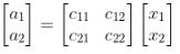
数值积分  scipy.integrate 

•  利用dir()获取你需要的信息
• 对自定义函数做积分

import scipy.integrate as si
from scipy.integrate import quad
import numpy as np
import matplotlib.pyplot as plt
f = lambda x:x**1.05*0.001
 
interval = 100
xmax = np.linspace(1,5,interval)
integral,error = np.zeros(xmax.size),np.zeros(xmax.size)
for i in range(interval):
    integral[i],error[i] = quad(f,0,xmax[i])
plt.plot(xmax,integral,label="integral")
plt.plot(xmax,error,label="error")
plt.show()

对震荡函数做积分

quad 函数允许 调整他使用的网格

>>>(-0.4677718053224297, 2.5318630220102742e-05)
>>>quad(np.cos,-1,1,limit=100)
>>>(1.6829419696157932, 1.8684409237754643e-14)
>>>quad(np.cos,-1,1,limit=1000)
>>>(1.6829419696157932, 1.8684409237754643e-14)
>>>quad(np.cos,-1,1,limit=10)
>>>(1.6829419696157932, 1.8684409237754643e-14)

微分方程的数值解 参见  Python数值求解微分方程方法(欧拉法,隐式欧拉)

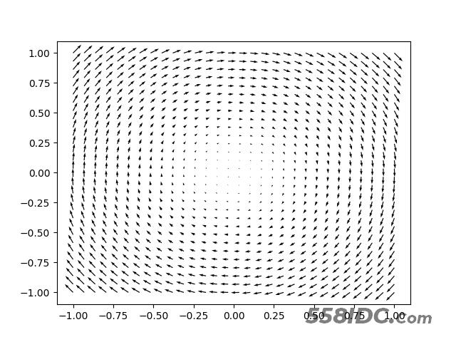
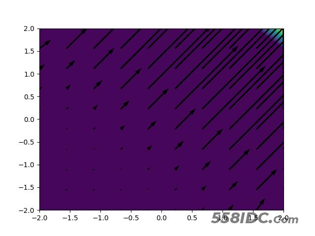
向量场与流线图：

vector(x,y) = (y,-x)  

import numpy as np
import matplotlib.pyplot as plt
coords = np.linspace(-1,1,30)
X,Y = np.meshgrid(coords,coords)
Vx,Vy = Y,-X
 
plt.quiver(X,Y,Vx,Vy)
plt.show()
------------------
import numpy as np
import matplotlib.pyplot as plt
 
coords = np.linspace(-2,2,10)
X,Y = np.meshgrid(coords,coords)
Z = np.exp(np.exp(X+Y))
 
ds = 4/6
dX,dY = np.gradient(Z,ds)
plt.contourf(X,Y,Z,25)
plt.quiver(X,Y,dX.transpose(),dY.transpose(),scale=25)
plt.show()

到此这篇关于Python数值方法及数据可视化的文章就介绍到这了,更多相关Python数值 视化内容请搜索自由互联以前的文章或继续浏览下面的相关文章希望大家以后多多支持自由互联！