1 简介 UKF 算法是广泛应用的非线性滤波方法之一, 在加性噪声条件下, 根据是否状态扩展和是否重采样有四种实现方式. 从算法精度、适应性和计算效率等方面进行了理论分析和仿真计算
1 简介
UKF 算法是广泛应用的非线性滤波方法之一, 在加性噪声条件下, 根据是否状态扩展和是否重采样有四种实现方式. 从算法精度、适应性和计算效率等方面进行了理论分析和仿真计算, 证明适当选择滤波器参数, 常用采样策略下, 状态扩展与非扩展的 UT 变换结果相同, 但后者的计算效率较高; 加性测量噪声条件下, 扩展与非扩展 UKF 可获得相同的滤波结果; 加性过程噪声条件下, 扩展与非扩展 UKF 仅能获得相同的状态预测结果; 重采样不总是构建滤波器的必要环节, 但理论分析和仿真计算发现了重采样对滤波器增益的自适应调节能力, 指出其在状态偏差或未知机动模式较大时对改善滤波器收敛性和精度有重要贡献.
 编辑
编辑
 编辑
编辑
 编辑
编辑
 编辑
编辑
2 部分代码
%% UKF bicycle testclear all
close all
% load params from file
load('bicycle_data.mat')
stop_for_sigmavis = true;
%% Data Initialization
x_pred_all = []; % predicted state history
x_est_all = []; % estimated state history with time at row number 6
P_est = 0.2*eye(n_x); % initial uncertainty
P_est(4,4) = 0.3; % initial uncertainty
P_est(5,5) = 0.3; % initial uncertainty
%% process noise
acc_per_sec = 0.2; % acc in m/s^2 per sec
yaw_acc_per_sec = 0.2; % yaw acc in rad/s^2 per sec
Z_l_read = [];
std_las1 = 0.15;
std_las2 = 0.15;
std_radr = 0.3;
std_radphi = 0.0175;
std_radrd = 0.1;
% UKF params
n_aug = 7;
kappa = 3-n_aug;
w = zeros(2*n_aug+1,1);
w(1) = kappa/(kappa+n_aug);
for i=2:(2*n_aug+1)
w(i) = 0.5/(n_aug+kappa);
end
%% UKF filter recursion
%x_est_all(:,1) = GT(:,1);
Xi_pred_all = [];
Xi_aug_all = [];
x_est = [0.1 0.1 0.1 0.1 0.01];
last_time = 0;
use_laser = 1;
use_radar = 0;
% load measurement data from file
fid = fopen('obj_pose-laser-radar-synthetic-ukf-input.txt');
%% State Initialization
tline = fgets(fid); % read first line
% find first laser measurement
while tline(1) ~= 'L' % laser measurement
tline = fgets(fid); % go to next line
end
line_vector = textscan(tline,'%s %f %f %f %f %f %f %f %f %f');
last_time = line_vector{4};
x_est(1) = line_vector{2}; % initialize position p_x
x_est(2) = line_vector{3}; % initialize position p_y
tline = fgets(fid); % go to next line
% counter
k = 1;
while ischar(tline) % go through lines of data file
% find time of measurement
if tline(1) == 'L' % laser measurement
if use_laser == false
tline = fgets(fid); % skip this line and go to next line
continue;
else % read laser meas time
line_vector = textscan(tline,'%s %f %f %f %f %f %f %f %f %f');
meas_time = line_vector{1,4};
end
elseif tline(1) == 'R' % radar measurement
if use_radar == false
tline = fgets(fid); % skip this line and go to next line
continue;
else % read radar meas time
line_vector = textscan(tline,'%s %f %f %f %f %f %f %f %f %f %f');
meas_time = line_vector{5};
end
else % neither laser nor radar
disp('Error: not laser nor radar')
return;
end
delta_t_sec = ( meas_time - last_time ) / 1e6; % us to sec
last_time = meas_time;
%% Prediction part
p1 = x_est(1);
p2 = x_est(2);
v = x_est(3);
yaw = x_est(4);
yaw_dot = x_est(5);
x = [p1; p2; v; yaw; yaw_dot];
std_a = acc_per_sec; % process noise long. acceleration
std_ydd = yaw_acc_per_sec; % process noise yaw acceleration
if std_a == 0;
std_a = 0.0001;
end
if std_ydd == 0;
std_ydd = 0.0001;
end
% Create sigma points
x_aug = [x ; 0 ; 0];
P_aug = [P_est zeros(n_x,2) ; zeros(2,n_x) [std_a^2 0 ; 0 std_ydd^2 ]];
%P_aug = nearestSPD(P_aug);
Xi_aug = zeros(n_aug,2*n_aug+1);
sP_aug = chol(P_aug,'lower');
Xi_aug(:,1) = x_aug;
for i=1:n_aug
Xi_aug(:,i+1) = x_aug + sqrt(n_aug+kappa) * sP_aug(:,i);
% figure(3)
% hold on;
% plot(GT(1,k), GT(2,k), '-og');
% plot(x_est(1,:), x_est(2,:), '-or');
% plot(Z_l(1,k), Z_l(2,k), '-xb');
% axis equal
% legend('GT', 'est', 'Lasermeas')
% k
tline = fgets(fid); % read the next line of the data file
end
fclose(fid);
Xi_pred_p1 = squeeze(Xi_pred_all(1,:,:));
Xi_pred_p2 = squeeze(Xi_pred_all(2,:,:));
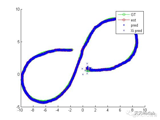
figure(2)
hold on;
plot(GT(1,:), GT(2,:), '-og');
plot(x_est_all(1,:), x_est_all(2,:), '-or');
plot(x_pred_all(1,:), x_pred_all(2,:), '.b');
plot(Xi_pred_p1, Xi_pred_p2, 'xb');
legend('GT', 'est', 'pred', 'Xi pred')
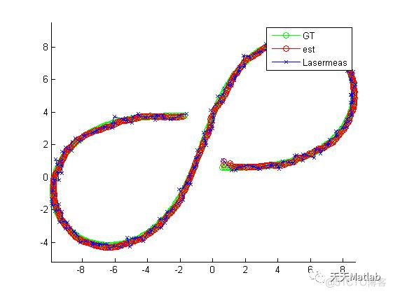
figure(3)
hold on;
plot(GT(1,:), GT(2,:), '-og');
plot(x_est_all(1,:), x_est_all(2,:), '-or');
plot(Z_l_read(1,:), Z_l_read(2,:), '-xb');
axis equal
legend('GT', 'est', 'Lasermeas')
%%
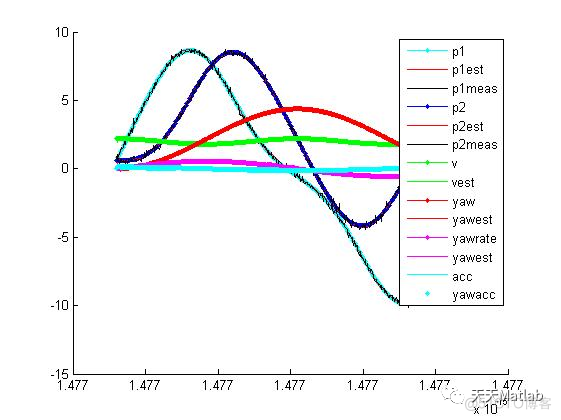
figure(1)
hold on;
plot(GT(8,:),GT(1,:), '.-c');
plot(x_est_all(6,:),x_est_all(1,:), '-r');
plot(Z_l(3,:),Z_l(1,:), '-k');
plot(GT(8,:),GT(2,:), '.-b');
plot(x_est_all(6,:),x_est_all(2,:), '-r');
plot(Z_l(3,:),Z_l(2,:), '-k');
plot(GT(8,:),GT(3,:), '.-g');
plot(x_est_all(6,:),x_est_all(3,:), '-g');
plot(GT(8,:),GT(4,:), '.-r');
plot(x_est_all(6,:),x_est_all(4,:), '-r');
plot(GT(8,:),GT(5,:), '.-m');
plot(x_est_all(6,:),x_est_all(5,:), '-m');
plot(GT(8,:),[0 diff(GT(3,:))/delta_t_sec], '-c');
plot(GT(8,:),[0 diff(GT(5,:))/delta_t_sec], '.c');
legend('p1', 'p1est','p1meas', 'p2', 'p2est','p2meas', 'v', 'vest', 'yaw', 'yawest', 'yawrate', 'yawest', 'acc', 'yawacc')
3 仿真结果
 编辑
编辑
 编辑
编辑
 编辑
编辑
4 参考文献
[1]杨旭升, 张文安, 俞立. 基于UKF算法的目标跟踪系统设计及实现[J]. 2013.
博主简介:擅长智能优化算法、神经网络预测、信号处理、元胞自动机、图像处理、路径规划、无人机等多种领域的Matlab仿真,相关matlab代码问题可私信交流。

 编辑
编辑