Excel怎么自动生成甘特图,很多朋友都遇到了这样的问题。这个问题该如何解决呢?下面小编就带来,希望可以帮到您! 1、如图所示,首先我们在excel表中输入如下数据。 2、然后我们
Excel怎么自动生成甘特图,很多朋友都遇到了这样的问题。这个问题该如何解决呢?下面小编就带来,希望可以帮到您!

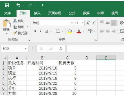
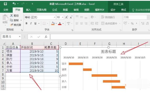
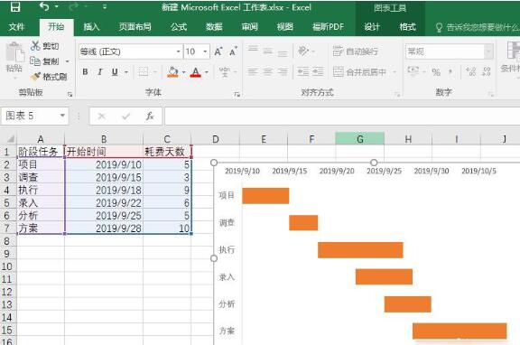
1、如图所示,首先我们在excel表中输入如下数据。
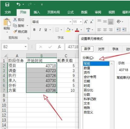
2、然后我们选中日期这列数据,将其单元格格式设置为常规。
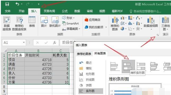
3、然后我们依此点击excel菜单栏的插入——图表——条形图——堆积条形图。
Excel相关攻略推荐:
excel怎么查找_excel查找方法指南
Excel中怎么求和 具体操作步骤介绍
Excel制作统计表格的操作步骤
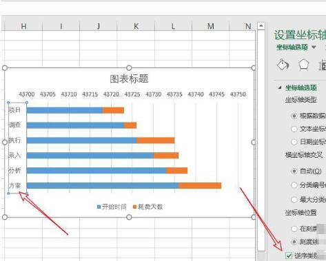
4、然后我们双击纵坐标——坐标轴选项,勾选逆序类别。
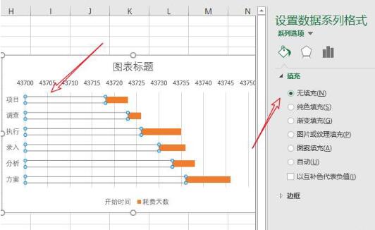
5、然后我们双击前面的蓝色条形柱,选择填充——无填充。
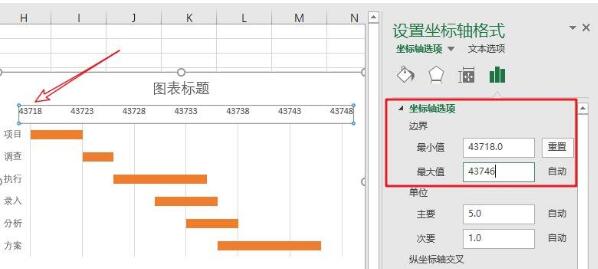
6、然后我们双击横坐标,点击设置坐标轴选项,最小值设置为步骤一开始时间的最小日期43718,最大值设置为最大日期+耗费天数(43736+10)。
7、然后我们将开始时间期设置单元格格式为日期,如图所示。
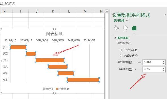
8、然后双击橙色条形柱,然后选择系列选项——分类间距,设置分类间距可以调整橙色条形柱的粗细,这里我们设置为70%。
9、最后,我们将一些不必要的如标题,图例删除,就做好一个简单的甘特图了。
以上就是Excel自动生成甘特图方式一览的全部内容了,自由互联为您提供最好用的浏览器下载,为您带来最新的软件资讯!