1 简介
In this paper, a modified particle swarm optimization (PSO) algorithm called autonomous groups particles swarm optimization (AGPSO) is proposed to further alleviate the two problems of trapping in local minima and slow convergence rate in solving high-dimensional problems. The main idea of AGPSO algorithm is inspired by individuals’ diversity in bird flocking or insect swarming. In natural colonies, individuals are not basically quite similar in terms of intelligence and ability, but they all do their duties as members of a colony. Each individual’s ability can be useful in a particular situation. In this paper, a mathematical model of diverse particles groups called autonomous groups is proposed. In other words different functions with diverse slopes, curvatures, and interception points are employed to tune the social and cognitive parameters of the PSO algorithm to give particles different behaviors as in natural colonies. The results show that PSO with autonomous groups of particles outperforms the conventional and some recent modifications of PSO in terms of escaping local minima and convergence speed. The results also indicate that dividing particles in groups and allowing them to have different individual and social thinking can improve the performance of PSO significantly.

2 部分代码
% Autonomous Groups Particles Swarm Optimization (AGPSO) source codes version 1.1 %% %
% Developed in MATLAB R2014a(7.13) %
% %
%
% You can simply define your cost in a seperate file and load its handle to fobj
% The initial parameters that you need are:
%__________________________________________
% fobj = @YourCostFunction
% dim = number of your variables
% Max_iteration = maximum number of generations
% SearchAgents_no = number of search agents
% lb=[lb1,lb2,...,lbn] where lbn is the lower bound of variable n
% ub=[ub1,ub2,...,ubn] where ubn is the upper bound of variable n
% If all the variables have equal lower bound you can just
% define lb and ub as two single number numbers
% To run AGPSO3: [Best_score,Best_pos,GWO_cg_curve]=AGPSO3(SearchAgents_no,Max_iteration,lb,ub,dim,fobj)
%__________________________________________
clear all
clc
SearchAgents_no=30; % Number of search agents
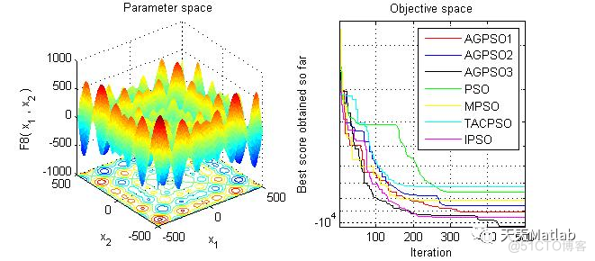
Function_name='F8'; % Name of the test function that can be from F1 to F23 (Table 1,2,3 in the paper)
Max_iteration=500; % Maximum numbef of iterations
% Load details of the selected benchmark function
[lb,ub,dim,fobj]=Get_Functions_details(Function_name);
[Best_score1,Best_pos1,AGPSO1_cg_curve]= AGPSO1(SearchAgents_no,Max_iteration,lb,ub,dim,fobj);
[Best_score2,Best_pos2,AGPSO2_cg_curve]= AGPSO2(SearchAgents_no,Max_iteration,lb,ub,dim,fobj);
[Best_score3,Best_pos3,AGPSO3_cg_curve]= AGPSO3(SearchAgents_no,Max_iteration,lb,ub,dim,fobj);
[Best_score4,Best_pos4,PSO_cg_curve] = PSO(SearchAgents_no,Max_iteration,lb,ub,dim,fobj);
[Best_score5,Best_pos5,IPSO_cg_curve]= IPSO(SearchAgents_no,Max_iteration,lb,ub,dim,fobj);
[Best_score6,Best_pos6,TACPSO_cg_curve]= TACPSO(SearchAgents_no,Max_iteration,lb,ub,dim,fobj);
[Best_score7,Best_pos7,MPSO_cg_curve]= MPSO(SearchAgents_no,Max_iteration,lb,ub,dim,fobj);
figure('Position',[300 300 660 290])
%Draw search space
subplot(1,2,1);
func_plot(Function_name);
title('Parameter space')
xlabel('x_1');
ylabel('x_2');
zlabel([Function_name,'( x_1 , x_2 )'])
%Draw convergence curves
subplot(1,2,2);
semilogy(AGPSO1_cg_curve,'Color','r')
hold on
semilogy(AGPSO2_cg_curve,'Color','b')
semilogy(AGPSO3_cg_curve,'Color','k')
semilogy(PSO_cg_curve,'Color','g')
semilogy(MPSO_cg_curve,'Color','y')
semilogy(TACPSO_cg_curve,'Color','c')
semilogy(IPSO_cg_curve,'Color','m')
title('Objective space')
xlabel('Iteration');
ylabel('Best score obtained so far');
axis tight
grid on
box on
legend('AGPSO1','AGPSO2','AGPSO3', 'PSO', 'MPSO', 'TACPSO', 'IPSO')
display(['The best solution obtained by AGPSO1 is : ', num2str(Best_pos1)]);
display(['The best optimal value obtained by AGPSO1 is : ', num2str(Best_score1)]);
display(['The best solution obtained by AGPSO2 is : ', num2str(Best_pos2)]);
display(['The best optimal value obtained by AGPSO2 is : ', num2str(Best_score2)]);
display(['The best solution obtained by AGPSO3 is : ', num2str(Best_pos3)]);
display(['The best optimal value obtained by AGPSO3 is : ', num2str(Best_score3)]);
display(['The best solution obtained by SPSO is : ', num2str(Best_pos4)]);
display(['The best optimal value obtained by SPSO is : ', num2str(Best_score4)]);
display(['The best solution obtained by MPSO is : ', num2str(Best_pos5)]);
display(['The best optimal value obtained by MPSO is : ', num2str(Best_score5)]);
display(['The best solution obtained by TACPSO is : ', num2str(Best_pos6)]);
display(['The best optimal value obtained by TACPSO is : ', num2str(Best_score6)]);
display(['The best solution obtained by IPSO is : ', num2str(Best_pos1)]);
display(['The best optimal value obtained by IPSO is : ', num2str(Best_score1)]);
3 仿真结果
4 参考文献
[1] Mirjalili S , Lewis A , Sadiq A S . Autonomous Particles Groups for Particle Swarm Optimization[J]. Arabian Journal for Science & Engineering, 2014, 39(6):4683-4697.
博主简介:擅长智能优化算法、神经网络预测、信号处理、元胞自动机、图像处理、路径规划、无人机等多种领域的Matlab仿真,相关matlab代码问题可私信交流。
部分理论引用网络文献,若有侵权联系博主删除。